Wavelet routine for multiple regression — wave.multiple.regression • wavemulcor

Produces an estimate of the multiscale multiple regression (as defined below) along with approximate confidence intervals.

wave.multiple.regression(xx, N, p = 0.975, ymaxr=NULL)

Arguments

xx	A list of \(n\) (multiscaled) time series, usually the outcomes of dwt or modwt, i.e. xx <- list(v1.modwt.bw, v2.modwt.bw, v3.modwt.bw)
N	length of the time series
p	one minus the two-sided p-value for the confidence interval, i.e. the cdf value.
ymaxr	index number of the variable whose correlation is calculated against a linear combination of the rest, otherwise at each wavelet level wmc chooses the one maximizing the multiple correlation.

Details

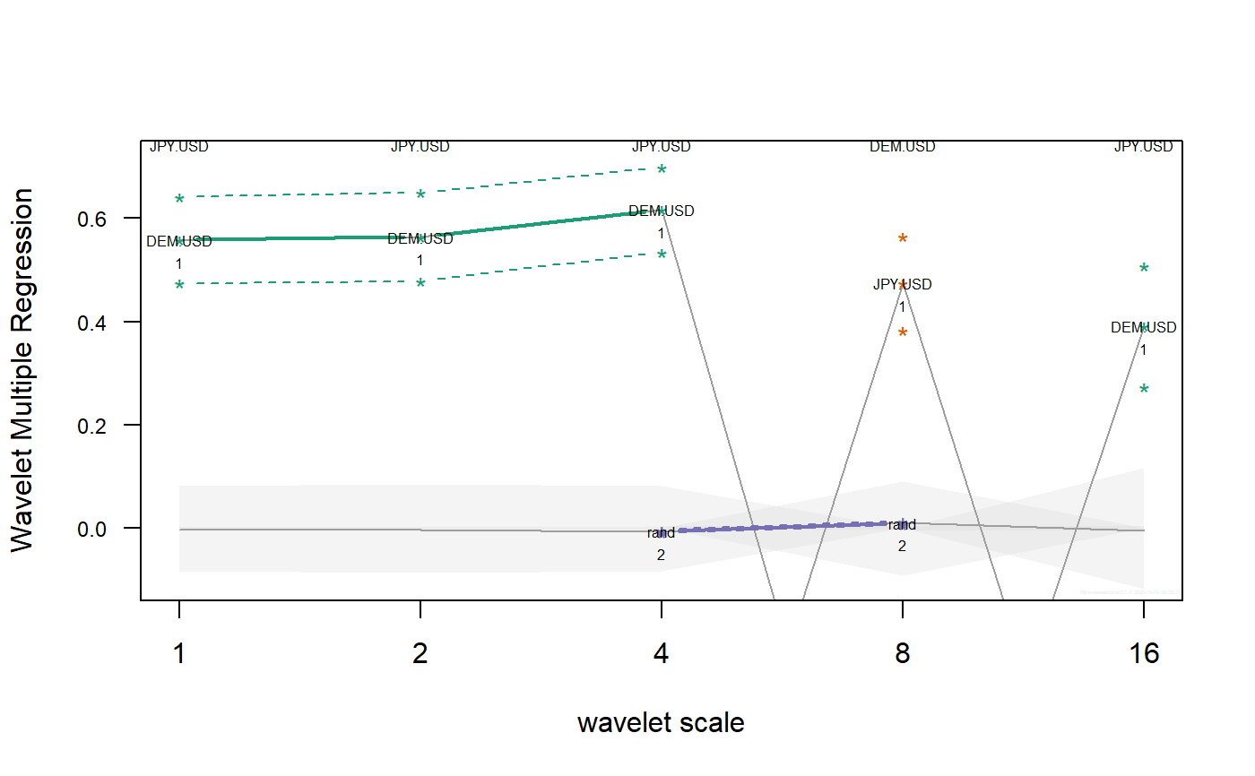
TThe routine calculates one single set of wavelet multiple regressions out of \(n\) variables that can be plotted in a single graph.

Value

List of four elements:

xy.mulcor:

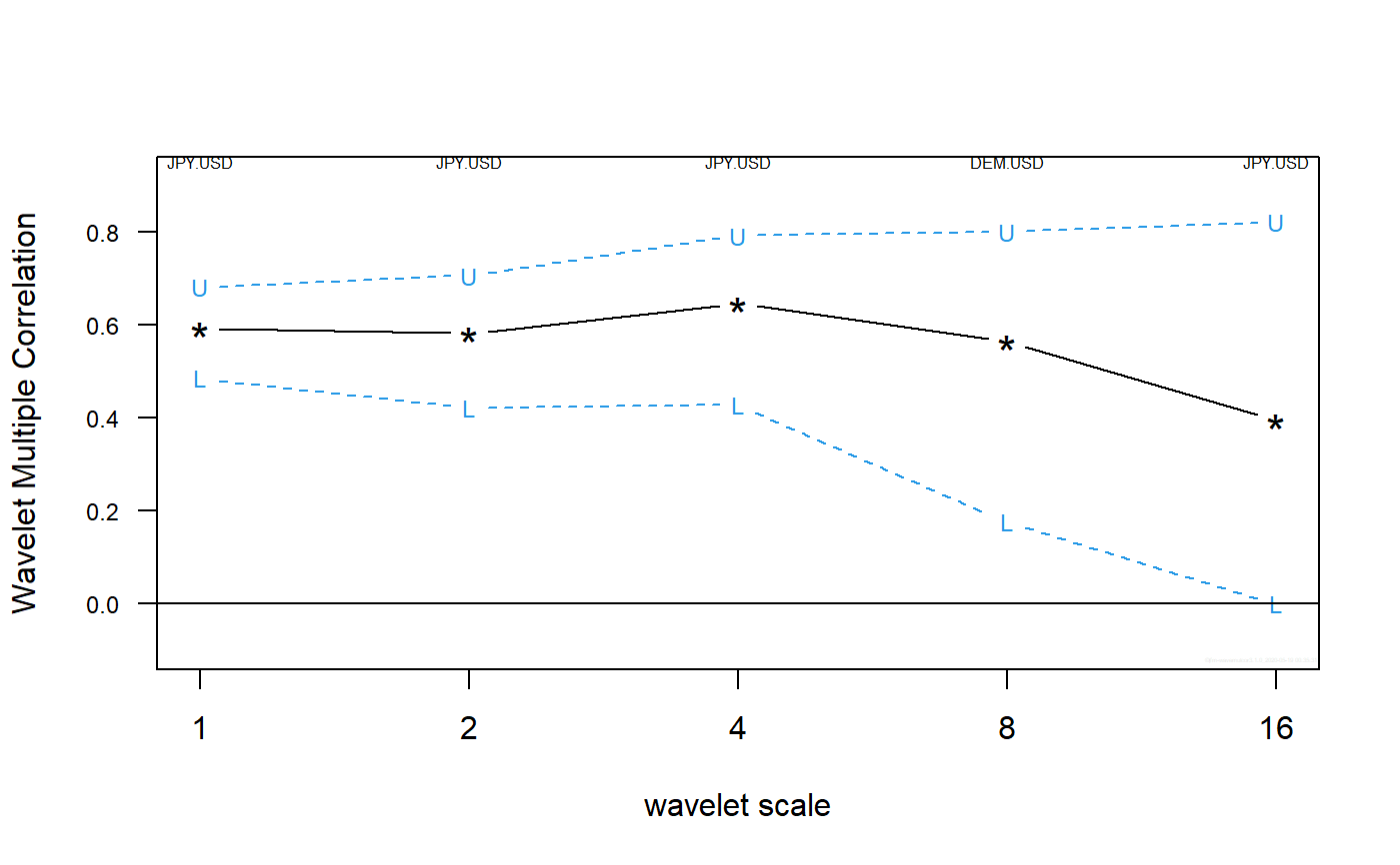
numeric matrix with as many rows as levels in the wavelet transform object. The first column provides the point estimate for the wavelet multiple correlation, followed by the lower and upper bounds from the confidence interval.

xy.mulreg:

List of seven elements:

rval: numeric matrix (rows = #levels, cols = #regressors+1) of regression estimates. rstd: numeric matrix (rows = #levels, cols = #regressors+1) of their standard deviations. rlow: numeric matrix (rows = #levels, cols = #regressors+1) of their lower bounds. rupp: numeric matrix (rows = #levels, cols = #regressors+1) of their upper bounds. rtst: numeric matrix (rows = #levels, cols = #regressors+1) of their t statistic values. rord: numeric matrix (rows = #levels, cols = #regressors+1) of their index order when sorted by significance. rpva: numeric matrix (rows = #levels, cols = #regressors+1) of their p values.

YmaxR:

numeric vector giving, at each wavelet level, the index number of the variable whose correlation is calculated against a linear combination of the rest. By default, wmc chooses at each wavelet level the variable maximizing the multiple correlation.

data:

dataframe (rows = #levels, cols = #regressors) of original data.

References

Fernández-Macho, J., 2018. Time-localized wavelet multiple regression and correlation, Physica A: Statistical Mechanics, vol. 490, p. 1226--1238. <DOI:10.1016/j.physa.2017.11.050>

Note

Needs waveslim package to calculate dwt or modwt coefficients as inputs to the routine (also for data in the example).

Examples

## Based on data from Figure 7.8 in Gencay, Selcuk and Whitcher (2001)
## plus one random series.

library(wavemulcor)

data(exchange)
returns <- diff(log(as.matrix(exchange)))
returns <- ts(returns, start=1970, freq=12)
N <- dim(returns)[1]

wf <- "d4"
J <- trunc(log2(N))-3

set.seed(140859)

demusd.modwt <- brick.wall(modwt(returns[,"DEM.USD"], wf, J), wf)
jpyusd.modwt <- brick.wall(modwt(returns[,"JPY.USD"], wf, J), wf)
xrand.modwt <- brick.wall(modwt(rnorm(length(returns[,"DEM.USD"])), wf, J), wf)

# ---------------------------

xx <- list(demusd.modwt, jpyusd.modwt, xrand.modwt)
names(xx) <- c("DEM.USD","JPY.USD","rand")

Lst <- wave.multiple.regression(xx)

# ---------------------------

##Producing correlation plot
plot_wave.multiple.correlation(Lst)
#> NULL

##Producing regression plot
plot_wave.multiple.regression(Lst)
#> NULL