Wavelet routine for multiple cross-regression

Produces an estimate of the multiscale multiple cross-regression (as defined below).

wave.multiple.cross.regression(xx, lag.max=NULL, p = .975, ymaxr=NULL)

Arguments

xx	A list of \(n\) (multiscaled) time series, usually the outcomes of dwt or modwt, i.e. xx <- list(v1.modwt.bw, v2.modwt.bw, v3.modwt.bw)
lag.max	maximum lag (and lead). If not set, it defaults to half the square root of the length of the original series.
p	one minus the two-sided p-value for the confidence interval, i.e. the cdf value.
ymaxr	index number of the variable whose correlation is calculated against a linear combination of the rest, otherwise at each wavelet level wmc chooses the one maximizing the multiple correlation.

Details

The routine calculates one single set of wavelet multiple cross-regressions out of \(n\) variables that can be plotted as one single set of graphs (one per wavelet level).

Value

List of four elements:

xy.mulcor

List of three elements:

wavemulcor: numeric matrix (rows = #levels, #cols = #lags and leads) with as many rows as levels in the wavelet transform object. The columns provide the point estimates for the wavelet multiple cross-correlations at different lags (and leads). The central column (lag=0) replicates the wavelet multiple correlations. Columns to the right (lag>0) give wavelet multiple cross-correlations with positive lag, i.e. with y=var[Pimax] lagging behind a linear combination of the rest: x[t]hat --> y[t+j]. Columns to the left (lag<0) give wavelet multiple cross-correlations with negative lag, i.e. with y=var[Pimax] leading a linear combination of the rest: y[t-j] --> x[t]hat. lower: numeric matrix (rows = #levels, #cols = #lags and leads) of lower bounds of the confidence interval. upper: numeric matrix (rows = #levels, #cols = #lags and leads) of upper bounds of the confidence interval.

xy.mulreg:

List of seven elements:

rval: numeric array (1stdim = #levels, 2nddim = #lags and leads, 3rddim = #regressors+1) of regression estimates. rstd: numeric array (1stdim = #levels, 2nddim = #lags and leads, 3rddim = #regressors+1) of their standard deviations. rlow: numeric array (1stdim = #levels, 2nddim = #lags and leads, 3rddim = #regressors+1) of their lower bounds. rupp: numeric array (1stdim = #levels, 2nddim = #lags and leads, 3rddim = #regressors+1) of their upper bounds. rtst: numeric array (1stdim = #levels, 2nddim = #lags and leads, 3rddim = #regressors+1) of their t statistic values. rord: numeric array (1stdim = #levels, 2nddim = #lags and leads, 3rddim = #regressors+1) of their index order when sorted by significance. rpva: numeric array (1stdim = #levels, 2nddim = #lags and leads, 3rddim = #regressors+1) of their p values.

YmaxR:

numeric vector giving, at each wavelet level, the index number of the variable whose correlation is calculated against a linear combination of the rest. By default, wmcr chooses at each wavelet level the variable maximizing the multiple correlation.

data:

dataframe (rows = #levels, cols = #regressors) of original data.

References

Fernández-Macho, J., 2018. Time-localized wavelet multiple regression and correlation, Physica A: Statistical Mechanics, vol. 490, p. 1226--1238. <DOI:10.1016/j.physa.2017.11.050>

Note

Needs waveslim package to calculate dwt or modwt coefficients as inputs to the routine (also for data in the example).

Examples

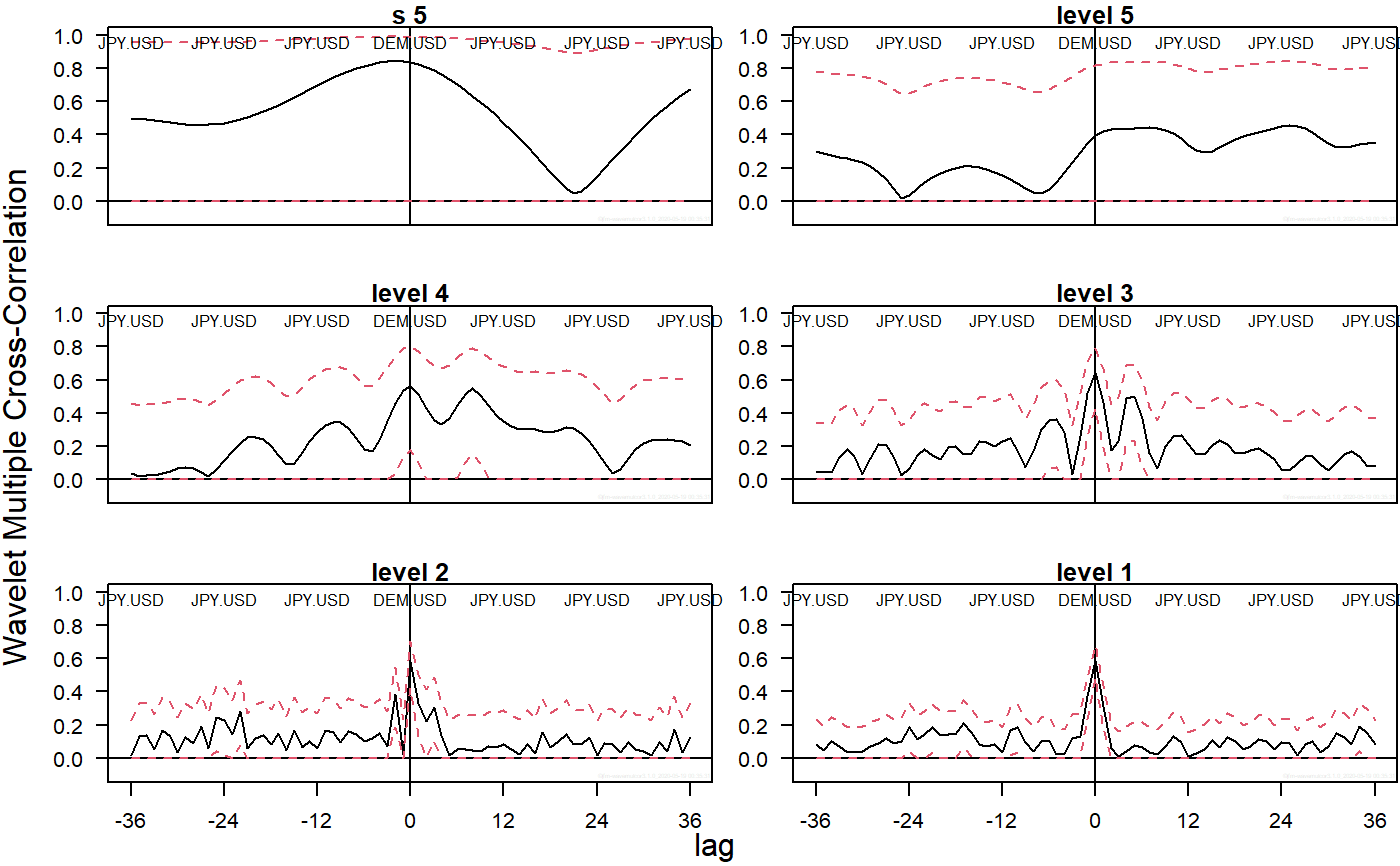
## Based on data from Figure 7.9 in Gencay, Selcuk and Whitcher (2001)
## plus one random series.

library(wavemulcor)

data(exchange)
returns <- diff(log(exchange))
returns <- ts(returns, start=1970, freq=12)
N <- dim(returns)[1]

wf <- "d4"
J <- trunc(log2(N))-3
lmax <- 36

set.seed(140859)

demusd.modwt <- brick.wall(modwt(returns[,"DEM.USD"], wf, J), wf)
jpyusd.modwt <- brick.wall(modwt(returns[,"JPY.USD"], wf, J), wf)
rand.modwt   <- brick.wall(modwt(rnorm(length(returns[,"DEM.USD"])), wf, J), wf)

# ---------------------------

xx <- list(demusd.modwt, jpyusd.modwt, rand.modwt)
names(xx) <- c("DEM.USD","JPY.USD","rand")

Lst <- wave.multiple.cross.regression(xx, lmax)

# ---------------------------

##Producing correlation plot

plot_wave.multiple.cross.correlation(Lst, lmax) #, by=2)
#> NULL

##Producing regression plot

plot_wave.multiple.cross.regression(Lst, lmax) #, by=2)
#> Error in plot_wave.multiple.cross.regression(Lst, lmax): object 'J' not found