Wavelet routine for local multiple regression — wave.local.multiple.regression • wavemulcor

Produces an estimate of the multiscale local multiple regression (as defined below) along with approximate confidence intervals.

wave.local.multiple.regression(xx, M, window="gauss", p = .975, ymaxr=NULL)

Arguments

xx	A list of \(n\) (multiscaled) time series, usually the outcomes of dwt or modwt, i.e. xx <- list(v1.modwt.bw, v2.modwt.bw, v3.modwt.bw)
M	length of the weight function or rolling window.
window	type of weight function or rolling window. Six types are allowed, namely the uniform window, Cleveland or tricube window, Epanechnikov or parabolic window, Bartlett or triangular window, Wendland window and the gaussian window. The letter case and length of the argument are not relevant as long as at least the first four characters are entered.
p	one minus the two-sided p-value for the confidence interval, i.e. the cdf value.
ymaxr	index number of the variable whose correlation is calculated against a linear combination of the rest, otherwise at each wavelet level wlmc chooses the one maximizing the multiple correlation.

Details

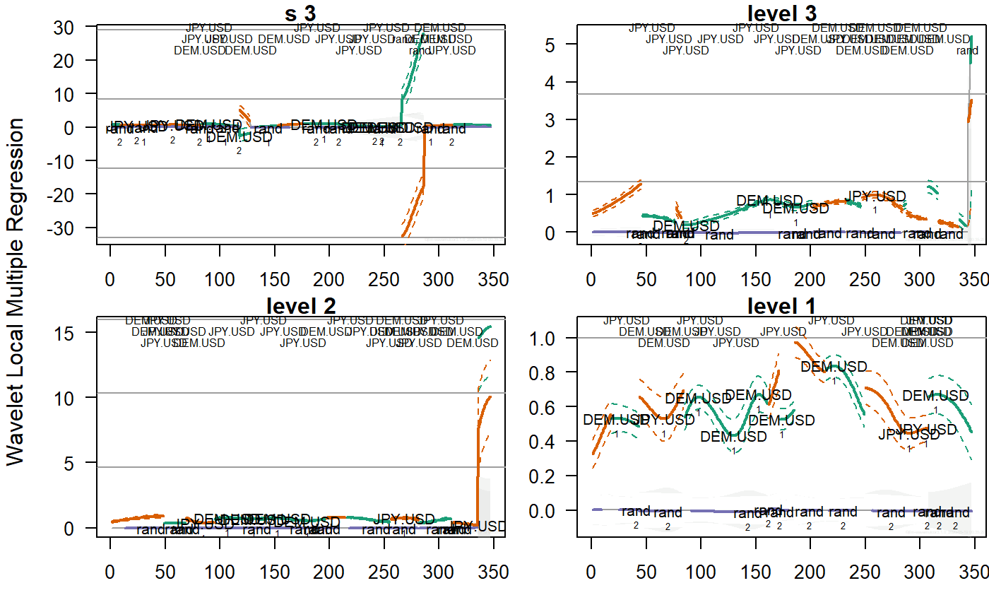
The routine calculates one single set of wavelet multiple regressions out of \(n\) variables that can be plotted in in \(J\) line graphs with explicit confidence intervals.

Value

List of four elements:

cor:

List of \(J+1\) elements, one per wavelet level, each with:

val: numeric matrix (rows = #observations, columns = #levels in the wavelet transform object) providing the point estimates for the wavelet local multiple correlation. lo: numeric matrix (rows = #observations, columns = #levels in the wavelet transform object) providing the lower bounds from the confidence interval. up: numeric matrix (rows = #observations, columns = #levels in the wavelet transform object) providing the upper bounds from the confidence interval.

reg:

List of \(J+1\) elements, one per wavelet level, each with:

rval: numeric matrix (rows = #observations, cols = #regressors+1) of local regression estimates. rstd: numeric matrix (rows = #observations, cols = #regressors+1) of their standard deviations. rlow: numeric matrix (rows = #observations, cols = #regressors+1) of their lower bounds. rupp: numeric matrix (rows = #observations, cols = #regressors+1) of their upper bounds. rtst: numeric matrix (rows = #observations, cols = #regressors+1) of their t statistic values. rord: numeric matrix (rows = #observations, cols = #regressors+1) of their index order when sorted by significance. rpva: numeric matrix (rows = #observations, cols = #regressors+1) of their p values.

YmaxR:

dataframe (rows = #observations, columns = #levels in the wavelet transform object) giving, at each wavelet level and time, the index number of the variable whose correlation is calculated against a linear combination of the rest. By default, wlmr chooses at each wavelet level and value in time the variable maximizing the multiple correlation.

data:

dataframe (rows = #observations, cols = #regressors) of original data.

References

Fernández-Macho, J., 2018. Time-localized wavelet multiple regression and correlation, Physica A: Statistical Mechanics, vol. 490, p. 1226--1238. <DOI:10.1016/j.physa.2017.11.050>

Note

Needs waveslim package to calculate dwt or modwt coefficients as inputs to the routine (also for data in the example).

Examples


## Based on data from Figure 7.8 in Gencay, Selcuk and Whitcher (2001)
## plus two random series.

library(wavemulcor)

data(exchange)
returns <- diff(log(as.matrix(exchange)))
returns <- ts(returns, start=1970, freq=12)
N <- dim(returns)[1]

wf <- "d4"
M <- 30
window <- "gauss"
J <- 3 #trunc(log2(N))-3

set.seed(140859)

demusd.modwt <- brick.wall(modwt(returns[,"DEM.USD"], wf, J), wf)
jpyusd.modwt <- brick.wall(modwt(returns[,"JPY.USD"], wf, J), wf)
xrand.modwt <- brick.wall(modwt(rnorm(length(returns[,"DEM.USD"])), wf, J), wf)

# ---------------------------

xx <- list(demusd.modwt, jpyusd.modwt, xrand.modwt)
names(xx) <- c("DEM.USD","JPY.USD","rand")

Lst <- wave.local.multiple.regression(xx, M, window=window) #, ymaxr=1)
#> 
#> lev:1234

# ---------------------------

##Producing line plots with CI

plot_wave.local.multiple.correlation(Lst) #, xaxt="s")

##Producing regression plots

plot_wave.local.multiple.regression(Lst) #, xaxt="s")
#> NULL