Routine for local multiple correlation
local.multiple.correlation.RdProduces an estimate of local multiple correlations (as defined below) along with approximate confidence intervals.
local.multiple.correlation(xx, M, window="gauss", p = .975, ymaxr=NULL)
Arguments
| xx | A list of \(n\) time series, e.g. xx <- list(v1, v2, v3) |
|---|---|
| M | length of the weight function or rolling window. |
| window | type of weight function or rolling window. Six types are allowed, namely the uniform window, Cleveland or tricube window, Epanechnikov or parabolic window, Bartlett or triangular window, Wendland window and the gaussian window. The letter case and length of the argument are not relevant as long as at least the first four characters are entered. |
| p | one minus the two-sided p-value for the confidence interval, i.e. the cdf value. |
| ymaxr | index number of the variable whose correlation is calculated against a linear combination of the rest, otherwise at each wavelet level lmc chooses the one maximizing the multiple correlation. |
Details
The routine calculates a time series of multiple correlations out of \(n\) variables. The code is based on the calculation of the square root of the coefficient of determination in that linear combination of locally weighted values for which such coefficient of determination is a maximum.
Value
List of four elements:
numeric vector (rows = #observations) providing the point estimates for the local multiple correlation.
numeric vector (rows = #observations) providing the lower bounds of the confidence interval.
numeric vector (rows = #observations) providing the upper bounds of the confidence interval.
numeric vector (rows = #observations) giving, at each value in time, the index number of the variable whose correlation is calculated against a linear combination of the rest. By default, lmc chooses at each value in time the variable maximizing the multiple correlation.
References
Fernández-Macho, J., 2018. Time-localized wavelet multiple regression and correlation, Physica A: Statistical Mechanics, vol. 490, p. 1226--1238. <DOI:10.1016/j.physa.2017.11.050>
Examples
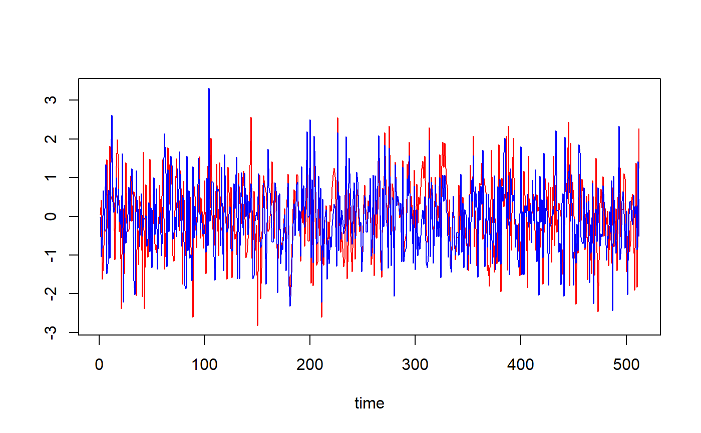
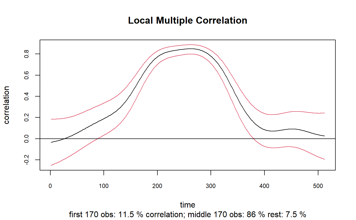
## Based on Figure 4 showing correlation structural breaks in Fernandez-Macho (2018). library(wavemulcor) options(warn = -1) xrand1 <- wavemulcor::xrand1 xrand2 <- wavemulcor::xrand2 N <- length(xrand1) b <- trunc(N/3) t1 <- 1:b t2 <- (b+1):(2*b) t3 <- (2*b+1):N wf <- "d4" M <- N/2^3 #sharper with N/2^4 window <- "gaussian" J <- trunc(log2(N))-3 # --------------------------- cor1 <- cor(xrand1[t1],xrand2[t1]) cor2 <- cor(xrand1[t2],xrand2[t2]) cor3 <- cor(xrand1[t3],xrand2[t3]) cortext <- paste0(round(100*cor1,0),"-",round(100*cor2,0),"-",round(100*cor3,0)) ts.plot(cbind(xrand1,xrand2),col=c("red","blue"),xlab="time")xx <- data.frame(xrand1,xrand2) # --------------------------- xy.mulcor <- local.multiple.correlation(xx, M, window=window) val <- as.matrix(xy.mulcor$val) lo <- as.matrix(xy.mulcor$lo) up <- as.matrix(xy.mulcor$up) YmaxR <- as.matrix(xy.mulcor$YmaxR) # --------------------------- old.par <- par() # ##Producing line plots with CI title <- paste("Local Multiple Correlation") sub <- paste("first",b,"obs:",round(100*cor1,1),"% correlation;","middle",b,"obs:", round(100*cor2,1),"%","rest:",round(100*cor3,1),"%") xlab <- "time" ylab <- "correlation" matplot(1:N,cbind(val,lo,up), main=title, sub=sub, xlab=xlab, ylab=ylab, type="l", lty=1, col= c(1,2,2), cex.axis=0.75)